
Alphabetizing in Excel by Last Name/Any Data
As with all things in Excel, there are multiple paths you can follow when alphabetizing in Excel. You can alphabetize a list or table of data including names. We explain three different methods in detail so you can find the one that works best for you. We show quick methods in brief; the fastest way is with only two clicks! We show in detail how to do a simple Sort, a Custom Sort and the powerful Filter. We quickly show how to alphabetize in brief immediately below, so read on.
Alphabetizing in Excel in Brief:
If you like shortcuts try this (if not read further below): Select a cell in the column in a range you want to sort, press <Alt> H S then S (to alphabetize) or O (to sort in reverse alphabetical order).
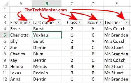
The image below shows how to alphabetize in Excel in one view.
Alternatively, with your range selected, you could press <Ctrl> <Shift> L at the same time, then click the down arrow and ‘Sort A to Z’. This is the method i use when quickly alphabetizing in Excel.
More detail for three methods with tips and notes below make it easier for you and help avoid pitfalls. If the above is not clear or you like to use a mouse and buttons (or touchscreen), or you want a little more guidance and explanation, read on.
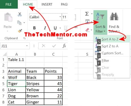
Alphabetizing in Excel, in one image.
This is a detailed guide. Suggest you click on the in-page link in the Contents below to take you direct to the section that seems most relevant to you.
Contents
How to – Alphabetizing in Excel in Brief
Alphabetizing in Excel – in Detail
Method 1 – Simple One-off Sort
Alphabetizing in Excel – Fastest way to Alphabetize (in Two Clicks!)
Using Only the Keyboard in Brief
How to Alphabetize in Excel 2 – Custom Sort (more capable)
Method 3 – Sort using a Filter (most powerful but quite simple)
Alphabetizing in Excel – in Detail
Again, there are several ways to do it; for each you can use the Ribbon or keyboard shortcuts.
Many people find clicking buttons with a mouse or using a touchscreen is easy. For this you can use the Ribbon.
Using the Ribbon menu (on a normal or large screen)
We want to show using the Ribbon as it is nice and visual with a mouse or touchscreen. We’ll show you keyboard shortcuts as we go. It is worth noting that the Ribbon does change depending on the size of the screen, so we’ll show whats required on a small screen further below.
We will explain what to do for a one-off Sort, how to use the more powerful Custom Sort button with its dialog box, and then we’ll show you how to set up a table Filter.
A Filter can do a lot more and is handy if you want to sort a large table in multiple ways. As the name suggests it can also filter out data (in many ways). It is very powerful because it can give more insights into your data.
How to Alphabetize in Excel – Method 1
Simple One-off Sort
This is the simplest way when alphabetizing in excel, showing how to alphabetize in Excel. Shown in detail so almost anyone can follow it.
Step 1: Select your table.
First, you need to help Excel know what you want to sort. Excel can identify a table automatically, so if you have one, just click in the table to select a cell anywhere in the column you want to alphabetize.
If you just have a single column, just click in that column. It is enough to have a cell selected anywhere in the column (as per image below).
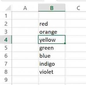
Ready to sort.
Some Notes and Tips for Selecting the Table (if easy for you, skip on down):
NOTE: to keep rows together when you sort, you want all the data in the row recognized or defined to be within one table. Similarly for columns.
NOTE: you want to notice whether Excel correctly determines if your list or table has a header row that you don’t want moved when you sort.
TIP: When your list is a short single column with a heading that looks similar to your list (e.g. text items and text header). Click and drag your mouse to select all the cells except your heading.
TIP: Inspect your results immediately after Alphabetizing. If Excel sorts including or excluding the top row you want or don’t want, press <Ctrl> z to undo.
NOTE: If you are using a Mac, use the Command key and letter shown instead of the <Ctrl> key described here and anywhere else in this article. I.e. <Command> z for undo, <Command> c for copy.
TIP: A more sophisticated method of sorting (shown further below) can give you the option to specify with a check box for ‘My data has headers’.
Excel is great because it remembers the table header correctly after you’ve helped it the first time.
Step 2: View the Home tab.
Click on the Ribbon ‘Home’ tab, if you are not already on it (click on or nearby the letters of the word HOME at the top of the screen).
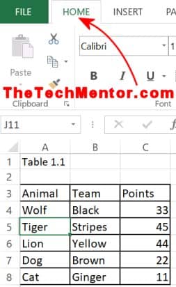
Home tab top left hand side.
If you want the keyboard shortcut, use the <Alt> key and letter H key.
You can tap on the screen on or nearby the letters of the word HOME if you have a touch screen.
NOTE: you will find ‘Sort and Filter’ buttons also in the Data tab on the Ribbon. The shortcut keys are a little different for that tab.
Step 3: Get the Sort and Filter Menu.
Click (or tap) ‘Sort and Filter’ button (shortcut <Alt> H S) in the ‘Editing’ group of buttons on the right hand side to show the menu.
Step 4: Select to Sort.
On the little drop down menu that appears, click on ‘Sort A to Z’ to alphabetize. Or just press the letter S on the keyboard at this point .
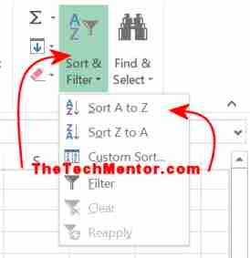
On the far right of the Ribbon in the ‘Editing’ tab, click Sort & Filter then Sort A to Z to alphabetize in Excel.
Alternatively, if you want to sort in reverse alphabetical order, click the next menu option down ‘Sort Z to A’ (or press the letter ‘o’ key on the keyboard).
TIP: to remember shortcut keys in the above steps is S is for Sort. Use the next letter of the word, o in sort to sort in reverse alphabetical order.
Alphabetizing in Excel – Fastest way to Alphabetize (in Two Clicks!).
If you’ve read above you understand some pitfalls and tips that might help this work best for you (due to header/no header).
Step 1: Right-Click in the table in the column you want to alphabetize.
TIP: The selected cell does not have to be in the table. Just right click directly in the column you want to sort.
Move the mouse down and hover over Sort in the pop up menu.
Step 2: When the subsequent menu pops up, click Sort A to Z.
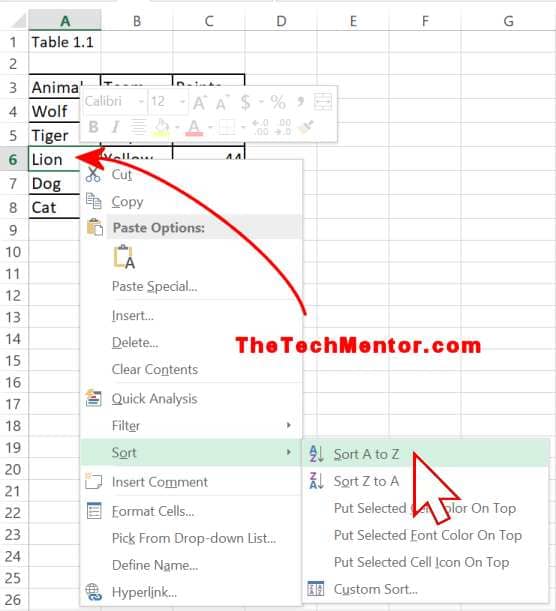
The fastest way to alphabetize in Excel – in two mouse clicks! First use the right mouse button.
The result of the above operation is as per the screenshot below.
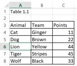
Excel table arranged alphabetically after we right-clicked in the first column.
Using Only the Keyboard in Brief
Many people who work on Excel a lot find using the keyboard quicker than the mouse (which can be fiddly for some).
Using only the keyboard, it is as follows:
Step 1: <Alt> H (for Home tab).
NOTE: you will see black letters appear on the Ribbon when you press <Alt>. Don’t be alarmed. These are the shortcut letters for all the options within the ribbon. They can be used for Accessibility so you don’t need a mouse.
Step 2: Now press S (for sort).
You press S for sort (you guessed it). Then…
Step 3: Choose whether to sort in forward or reverse order.
Then press S (for Sort A to Z) or O (for sort Z to A).
TIP: you don’t need to hold the <shift> key down as you select letters in the shortcut.
So you can press <Alt> h, s and finally s or o to alphabetize or sort in reverse alphabetical order respectively.

Excel keyboard shortcuts to alphabetize (start with H).
How to Alphabetize in Excel – Method 2
Custom Sort (More Capable)
This is a more complex method than the first to alphabetize in Excel.
Many people find Method 3 further below easier than this.
Importantly, a Custom Sort sorts alphabetically and keeps rows together.
NOTE: to keep rows together you want all the data in the row recognized or defined to be within one table. Same for columns.
FAQ:
How do I sort alphabetically in Excel without mixing data?
That typically means to keep rows together when you sort. The fix is do not have totally empty rows between parts of the data you want to be treated as a single table. Similarly, do not have totally empty Columns between your data that you don’t want mixed.
TIP: Where you would like to force Excel to treat your data as a single table and therefore not mix data, you can highlight all the data (yes, the whole data table) before you act to sort it.
We’ll manage Headers more easily with this method. You could check the start of Method 1 for details, tips and notes relating to selecting your table or column and headers.
Custom Sort is more capable than a simple Sort because you can sort a table by one column and by subsequent columns in one operation. However some find it a little more fiddly and complicated to use. That’s why some people prefer to use a Filter, because it is far more powerful with additional features and isn’t really much more complicated.
A Custom Sort is helpful when some of your items are identical and you want to define how these rows with common items will sort based on other columns (of text or data).
For example, you have names of children in a school and there are twins or triplets! We will show how to alphabetize last names in excel, and for the rows arranged together by identical last name, sort those by first name.
Step 1: Check you are on or click on the Home tab on the Ribbon.
Or use <Alt> H on the keyboard.
NOTE: You could alternatively use the Data tab, where the Sort & Filter group is.

Custom Sort step 1.
Step 2: Click on the Sort & Filter button towards the far right of the Ribbon.
Or if you started via the shortcut, continue with S (or ‘s’, i.e. no <shift> key required).
Step 3: When the drop down menu appears, click on ‘Custom Sort…‘.
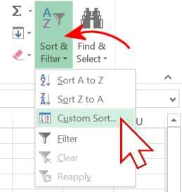
First click Sort and Filter, then Custom Sort… on Excel Ribbon.
To continue the shortcut, type U (or ‘u’).
Step 4: Notice and Adjust the Header Check Box.
In my example (shown below), the selected cell had been the top first row and column of the table. Excel automatically identified my table has a header and checked the ‘My Data Has Headers’ and selected the range within the table.
You can click the check box to toggle it on or off and observe the range selected in the table.
Alternatively you can type H to toggle it.
You will see something else brilliant Excel has also done in the background in the next step.
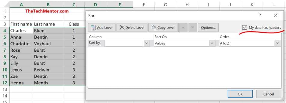
The Custom Sort set up box. Notice the header checkbox was pre-selected by Excel. I didn’t need to do it!
Step 5: Choose Last Name
Click the edit box’s little down arrow next to Sort by (under Column) and select to alphabetize by last name.
TIP: as seen in the image below, Excel pre-populated the drop down list with all the table header names. This is much clearer than Column A, Column B, Column C, etc. that appear when you don’t have a header row. Much clearer and easier to use. Brilliant!
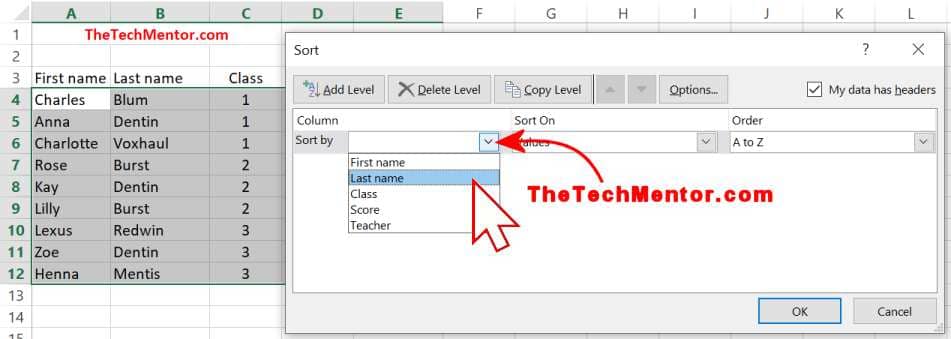
Excel pre-populated the drop down list with the names in my table header. It makes it nice and clear by what you choose to sort.
We can leave Sort On Values and Order A to Z as these defaults are what we need.
But what do we do with the twins? How do we tell Excel how we want those treated? We need to set up another level to sort by.
Step 6: Add a Sub-level by which to Sort (Optional).
Click Add Level and observe an additional row has been inserted under the first.
Then Click Sort by down arrow and select another option. For our example we choose First name.
Again, we leave Sort On Values and Order A to Z as these defaults are what we want.
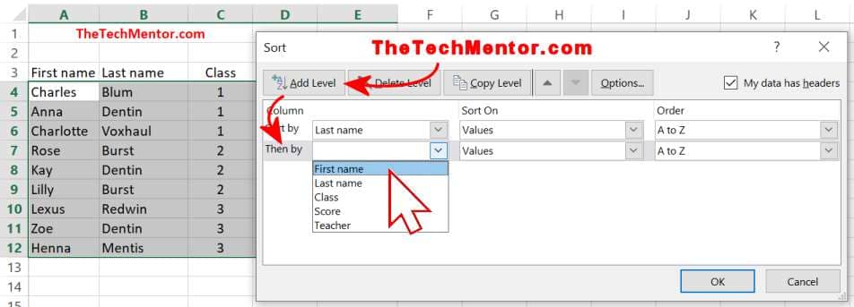
Custom sort with two levels of alphabetization by last name at the top level and then by first name as a secondary level.
TIP: In some situations we might want to organize by ascending numbers or some other arrangement after we alphabetize the top level names. For example, we could define a secondary sort by Class number for children with the same last name.
Step 7: Click OK or press <Enter>.
The Custom Sort setup form closes and the table is organized alphabetically by last name then by first name.

Here’s the result of our example custom sort to alphabetize by last name, then first name. Check out the order of the twins and triplets.
TIP: As for the simple Sort, you can instead right-click within the table to get a pop up menu, hover the mouse over Sort…, and then select Custom Sort at the end of the subsequent popup menu. From there you continue as above to set how you Excel to arrange your data.
If we change our mind and want to say, sort by class first, then by last name we could run custom sort again.
However, if we expect we will want to slice and dice our data in different ways to get better insights, we do not have to run Custom Sort over and over. With many variables it can become cumbersome. The solution is to use the very powerful table Filter.
Method 3 – Alphabetize in Excel Using a Filter (powerful but quite simple)
This method shows how to alphabetize in Excel with a filter which is a commonly used and quite simple method once you get the hang of it.
Table Filters are great because you can sort by data in any column when you have several columns of data.
This is very handy if, for example, you have a table that includes first and last names and want to alphabetize by last names one moment, by the names another moment, or by numeric data such as sales volumes, or by ascending dates, etc.
The bonus is you have other filter features as the name suggests. It’s a very powerful tool but all aspects of the Filter in Excel is beyond the scope of this article.
NOTE: If you are working on Excel spreadsheets from others (e.g., in a team) then your data might already have a Filter.
FAQ:
How to recognize if my Excel table already has a filter?
Look at the top (or header) row. At the end of each cell there would be a small box with a down arrow if a Filter is already applied. See screenshot below.
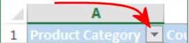
A Filter ads a small box with down arrow at the end of each header cell.
Step 1: Select your table.
If you have a clear set of data in a table, you can let Excel automatically select the whole table.
- You can click to select any cell inside the table (before you continue as below) and see if Excel does the rest as you want.
- Rows or columns right next to your table might make Excel include them as part of your table.
TIP: Insert a Row or Column to separate data you want included from other entries in your spreadsheet that you don’t want mixed up. - You can use <Ctrl> z to undo if it doesn’t work how you’d like.
Otherwise, to select (and define) your table to Excel, click and drag the mouse from the first cell in one corner to the last cell in the opposite corner to highlight all cells.
Step 2: Click to get the Sort and Filter menu.
Click on the Sort & Filter button on the Home tab of the Ribbon at the top of the screen.
Or type <Alt> H, then S on the keyboard.
Step 3: Select Filter.
When a drop-down menu appears, click on Filter (it has an icon that looks like a funnel).
Or you can type F rather than clicking the button.
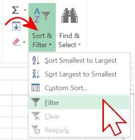
Filter on Excel Ribbon at the top right-hand side.
NOTE: There is a single shortcut to set a Filter when you have a cell selected in a table. Press <Ctrl> <Shift> L (all at the same time).
Every header cell has the small box and down arrow to access a drop down menu.
Notice at the header row of your table, each cell has a little box with a small down arrow.
These are controls that you use to manipulate the data. That includes the controls to sort your data alphabetically, sort smallest to highest for numbers, or filter (or hide) certain data and a whole lot more.
It might cover your header name. It can bother some people as it might be more difficult to read your header.
TIP: if you prefer to see the whole header name, adjust the column width (drag the end of the column label at the top, A, B, C etc. further to the right with the mouse) until the column is wider than the header name by the width of the little drop-down arrow box.
Step 4: Choose the column you want to alphabetize.
Click the drop-down button (down arrow) atop the table for that column.
A drop-down menu will appear with the next options.
Step 5: Click to Sort.
To begin alphabetizing in your Excel table, click Sort A to Z at the top of the drop-down menu.
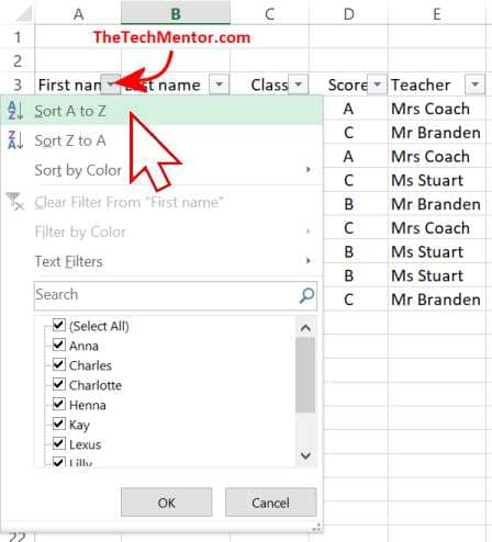
There are many more options that cen be seen in the drop-down menu. We only need the very top one to Alphabetize by first name in our example.
TIP: To sort alphabetically in reverse order, click the down arrow then click Sort Z to A second to top in the drop down menu that appears.
The Result – We have Alphabetized in Excel
The table will be sorted alphabetically for the column in which you selected the drop-down button. Notice each entire table row moves to keep the relevant data adjacent to the cell that has been sorted.
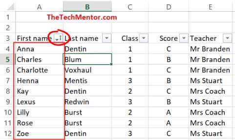
Our list sorted by First Name. Notice the drop-down button has changed to include a little arrow to show the entire table is sorted by this column.
NOTE: If you get a result you didn’t expect, it might be due to Excel incorrectly identifying your table, or your table header. You might need to make sure you have a blank row (or column) before your table starts. Or you might need to select the specific cells to which you want Excel to apply the Filter.
TIP: You can click undo (or use <Ctrl> z as the keyboard shortcut for undo) after you click Filter or after any sort step.
How to Alphabetize by Last Name then First Name with a Filter
Follow the above method Steps 4 and 5 to sort by first name, except that finally you click on the drop-down button in the Last Name header.
In our result below, we have alphabetized by Last Name.
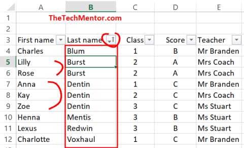
The drop down button has changed for the Last name.
Notice how the rows with the same last name (for the twins and triplets) have remained sorted alphabetically by first name.
NOTE: The excel filter keeps rows for identical items sorted in the order they were previously.
For a Filter, this is how to achieve the Custom Sort’s multiple ‘Level’ effect (shown above).
TIP: To get the above result if say, the school data were originally sorted by class, we should first sort by First Name, and only after that alphabetize by Last Name (as shown above).

Leave A Response